How Bucketeer A/B Test Choose Which Version of Your Feature to Ship

Hi, I’m a backend engineer working on Bucketeer, an open-source feature management and experimentation platform.

While investigating and debugging the product, I wanted to understand how our A/B testing actually worked, but there was no document explaining the logic in our repo before, it lived in a Stan model and some Go code. So I studied it and finally wrote up the documentation for the team. I find it interesting so I want to write this blog to share how the platform does it.

The goal is to open up the part that often gets treated as a black box: when you run an A/B test, how does the platform actually decide which variation is the winner?

To keep things clear, two layers stay separate throughout: first the general idea behind A/B testing, and then how Bucketeer applies that method by steps. This blog will not contain any mathematical equation or concept but the plain idea behind.

A. The question behind every A/B test

Take a simple example: we’re testing how to display a product’s price on its detail page. The product costs $50 either way — the amount charged at checkout never changes, only how the price looks on the page:

• Version A (plain price) simply shows $50.
• Version B (discount frame) shows the same $50 next to a crossed-out $60, so it reads as “was $60, now $50 and you save $10”.

We split traffic 50/50, and “converted” means the user bought. After a while we have this:

Variation	Users saw it	Converted	Observed conversion rate
A (Plain price)	10,000	500	5.0%
B (Discount frame)	10,000	600	6.0%

At first glance, B wins: 6.0% of users who saw the discount framing bought, versus 5.0% for the plain price. But 6.0% vs 5.0% from a single test run doesn’t prove B is truly better. Maybe B just got lucky with the users it happened to receive. If we re-ran the same test tomorrow, would B win again, or would the numbers flip?

That question, separating a real effect from random noise, is what the Experiment Calculator exists to answer.

B. How Bucketeer answer the question

The raw rates (5.0% vs 6.0%) don’t answer the real questions on their own:

• Which variation is probably better?
• How confident can we be?
• If we pick one and it’s worse, what does that cost?

Step 1 – Treat each rate as a range. A rate of 6% measured from 100 users and the same 6% measured from 10,000 users look identical, but we should trust them differently. To capture that, Bucketeer does not work with a single rate for each variation. It works with a range of rates the data is consistent with. When there is a lot of data that range is tight and sits close to the observed rate, and when there is little data it is wider, because the true rate could reasonably be higher or lower than what we happened to measure.

Step 2 – Compare the ranges by trying it. To compare two ranges, Bucketeer picks a random rate for A from its range and a random rate for B from its range, and checks which one is higher. It repeats this 100,000 times. The fraction of those tries where B comes out higher is B’s probability of being better, a real number, not a yes/no answer.

What the simulation does.

Trying it many times with random values like this is called a Monte Carlo simulation: you estimate an answer by running a large number of random trials and looking at how they turn out.

To make it concrete, switch to a different example for a moment. Say we run a gym and want to design a program for people who are brand new to lifting. The question is which first-week target weight sets beginners up to succeed, so we test two versions of the program, each on its own group of 100 new lifters:

• Program 1 — 20kg target: 22 of the 100 beginners can lift it by the end of the first week.
• Program 2 — 15kg target: with the lighter weight, 60 of the 100 can.

The trouble with plain randomness is that it has no memory. If we estimate the 20kg program’s true rate by making completely independent guesses, one trial might say 90 out of 100 similar beginners would succeed, the next 10, the next 70. For a group of similar people that is not very realistic, we already saw 22 out of 100, so a true rate near 90% or near 10% doesn’t match what we observed. Independent guesses spend most of their effort on values the data already points away from.

Markov Chain Monte Carlo (MCMC) fixes this by giving each guess a memory of the one before it. It starts near what we observed and takes a small random step each time, and it holds on to a step more readily when the new value still fits the data. So instead of swinging from 90 to 10, the chain of guesses for the 20kg program moves gently 22, then 30, then 25, then 18 and so on, … staying in the region the data supports. Collect all the values the chain visits and you have the range from Step 1. Bucketeer runs 100,000 of these steps for each variation.

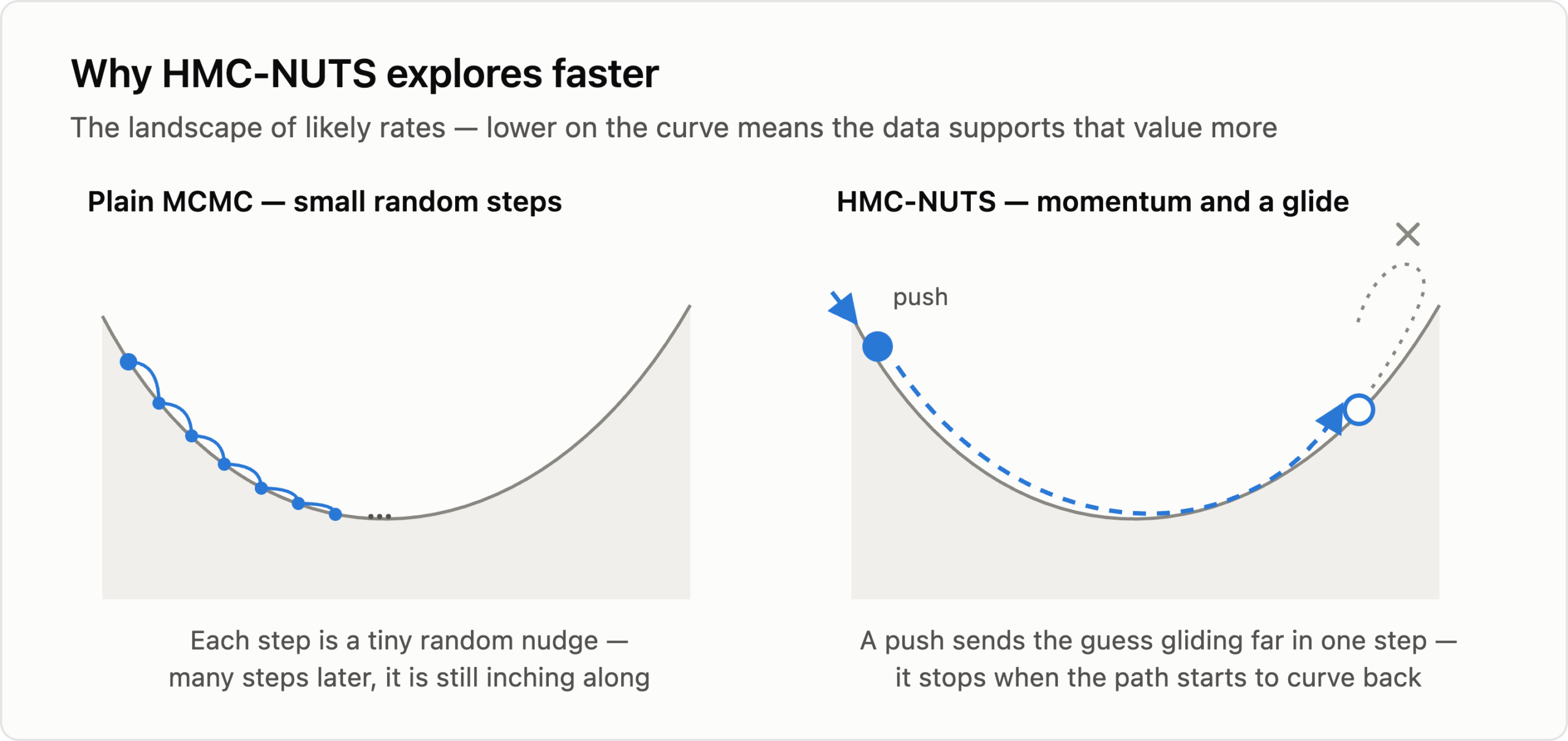
The exact method Bucketeer uses is called HMC-NUTS (short for Hamiltonian Monte Carlo with a No-U-Turn Sampler), which is just a more efficient way of choosing those steps.Picture the range of likely rates as a landscape where the better values sit in low valleys. Instead of nudging the current guess in a random direction, it gives the guess a small push and lets it roll along the slope, like a ball with a bit of momentum, so it can move a fair distance to another good value in one step rather than inching along. It also decides on its own how far to let the ball roll each time, stopping when the path starts to curve back on itself, so nothing has to be tuned by hand. The result is that the chain covers the range faster and needs fewer steps to settle.

The two numbers Bucketeer reports

Both come out of those draws.

The first is the probability of being best: how often each variation came out highest across the 100,000 tries. If B was highest in 99,800 of them, its probability of being best is 99.8%.

The second is the expected loss: if you pick a variation and it turns out not to be the best, how much you give up on average. For each try, Bucketeer measures the gap between the variation you picked and whichever one was actually highest that time, and then averages those gaps. In our example B’s expected loss is 0.02% and A’s is 1.0%, so picking B risks almost nothing while picking A risks about a percentage point of conversions.

The decision rule is simply to pick the variation with the lowest expected loss.

One guardrail: SRM

If the traffic split itself is off, the results on top of it can be misleading. You set up 50/50, but a bucketing bug or bot traffic makes it run 53/47.

Sample Ratio Mismatch (SRM) detection watches for this: Bucketeer checks whether the observed users per variation match the split you configured. If they differ more than chance can explain, it raises a warning rather than take the numbers at face value.

That’s the whole idea. In short, Bucketeer reaches a verdict by modelling each variation’s true rate, simulating which one is best, and reporting the probability and the expected loss, while setting the result aside if the traffic split looks off.

C. The calculation, step by step

Now let’s run the price test from the beginning through the actual calculation, with numbers. Below is the whole pipeline at a glance.

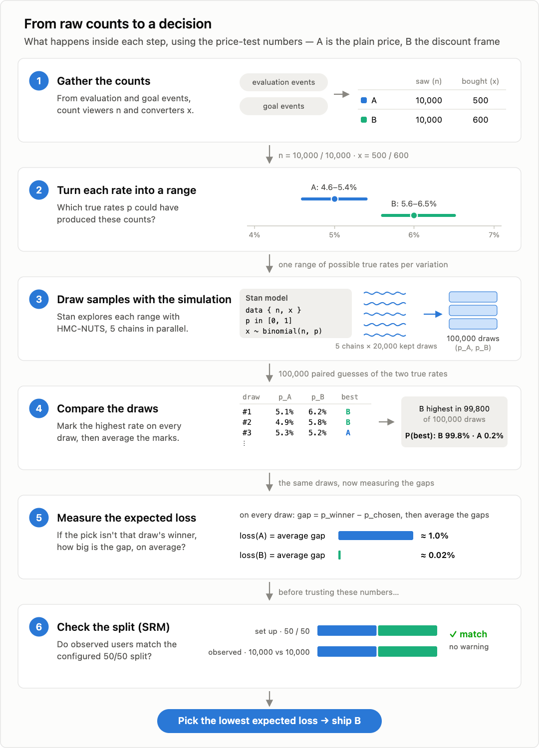
1. Gather the counts. For each variation Bucketeer needs two things: how many users saw it, and how many of them bought. The first comes from evaluation records, one is logged whenever a user is shown a variation. The second comes from goal records, one is logged when a user completes the action we’re measuring, which here is a purchase. For our test, 10,000 saw the plain price and 500 bought, and 10,000 saw the discount frame and 600 bought, the 5.0% and 6.0% from the table.
2. Turn each rate into a range. From those counts Bucketeer works out the range of true rates each result is consistent with. With 10,000 users behind each side, both ranges are fairly tight: the plain price sits around 4.6%–5.4%, and the discount frame is around 5.6%–6.5%.
3. Draw samples with the simulation. The sampling is done by a small model written in Stan, a language built for this kind of probability model. The whole thing is short:
   

   data {
       int g;      // number of variations
       int n[g];   // users who saw each variation
       int x[g];   // users who converted in each
   }
   
   parameters {
       real<lower=0, upper=1> p[g];   // the unknown true rate of each variation
   }
   
   model {
       for (i in 1:g)
           x[i] ~ binomial(n[i], p[i]);   // how conversions relate to the rate
   }
   
   generated quantities {
       for (i in 1:g)
           prob_best[i] = (p[i] is the highest of all p) ? 1 : 0;  // who won this draw
   }

   Read plainly, it says: given that n users saw a variation and x of them converted, which values of the true rate p could have produced that? Because p is only allowed between 0 and 1 with nothing else assumed, every rate starts out equally likely. Stan explores the answer with the HMC-NUTS steps from earlier, and on every draw it also marks which variation was highest (prob_best).
   The Go side that drives Stan is binomialModelSample. In pseudocode we can express it like this:
   

   binomialModelSample(n, x):
       run 5 chains in parallel:
           for each chain:
               send { g, n, x } to Stan, asking for HMC-NUTS sampling
               take 21,000 draws, discard the first 1,000 as warm-up
               keep the remaining 20,000
       merge the chains  ->  100,000 draws of (p, prob_best)
       return the draws

   So each draw pairs one possible rate for the plain price with one for the discount frame, 100,000 pairs in all.

4. Compare the draws. Averaging the prob_best marks across the 100,000 draws gives each variation’s probability of being best. The discount frame is highest in about 99,800 of them, so its probability of being the better price is 99.8%, and the plain price’s is 0.2%.
5. Measure the expected loss. For each draw it also records how far each variation sits below the higher one that time, then averages. The plain price’s expected loss works out to about 1.0% and the discount frame’s to about 0.02%, so choosing the discount frame risks almost nothing while choosing the plain price leaves roughly a percentage point of purchases behind.
6. Check the split. Finally it confirms the traffic ran the way we set it up. We configured 50/50, and 10,000 versus 10,000 matches that, so SRM raises no warning.Putting it together:
   

   Metric	A (Plain price)	B (Discount frame)
   Saw it / bought	10,000 / 500	10,000 / 600
   Observed rate	5.0%	6.0%
   Probability of being best	0.2%	99.8%
   Expected loss	1.0%	0.02%

   The discount frame is the better price with 99.8% confidence, choosing it risks almost nothing, and the split is clean, so it’s the one to ship.

   D. Wrapping up

   That’s the whole path, from raw counts to a decision: treat each rate as a range, draw a hundred thousand samples from it, compare them to get a probability of being best and an expected loss, and check the traffic split before trusting any of it.

   To dig deeper and read the full Bayesian math, the value-based metrics, the convergence checks, and the details of SRM, or read the full implementation, it’s all in: 

   • Bucketeer source code: https://github.com/bucketeer-io/bucketeer
   • Want to try it out? Let’s visit https://app.bucketeer.io and run your experiments in our demo environment

   References

   • Monte Carlo Markov Chain in the Stan Reference Manual: https://mc-stan.org/docs/reference-manual/mcmc.html
   • httpstan on GitHub: https://github.com/stan-dev/stan